
Bayesian Theory
A Bayesian problem consists of:
- Parametric model $p(\mathbf{x}|\mathbf{z})$: joint distributions of the observations $\mathbf{x}$ given the parameters and latent variables $\mathbf{z}$. It models our beliefs on how the data was generated given $\mathbf{z}$. $\mathbf{z}$ represent the non observed variables that governs the generation of observations.
- Prior distribution $p(\mathbf{z})$: The presumed density of the parameters $\mathbf{z}$. It models our beliefs on how the parameters look like.
Bayes' Theorem
Variational Inference
Variational Autoencoder
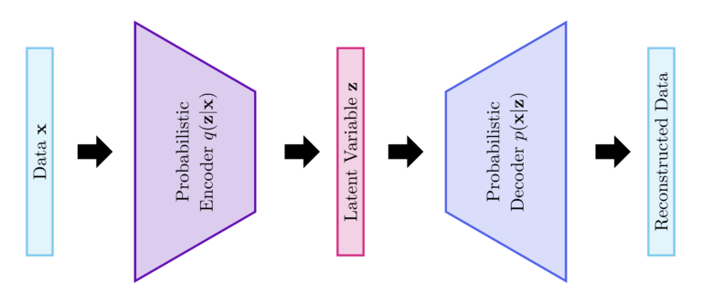
In variational autoencoders, the encoder learns $q(\mathbf{z}|\mathbf{x})$ to approximate $p(\mathbf{z}|\mathbf{x})$ while the decoder learns $p(\mathbf{x}|\mathbf{z})$. Please note that the decoder is the inverse of the encoder according to Bayes rule. The parameters of $q(\mathbf{z}|\mathbf{x})$ and $p(\mathbf{x}|\mathbf{z})$ are modeled using neural networks. In particular, the parameters of $q(\mathbf{z}|\mathbf{x})$ (resp. $p(\mathbf{x}|\mathbf{z})$) are the weights and biases of the encoder (resp. the decoder).
ELBO
The objective function optimized for the variational approximation is called the evidence lower bound and is defined as:
$$\mathcal{L}(\mathbf{x}) = \mathbb{E}_q\Big[\log\big(p(\mathbf{x}, \mathbf{z}) \big) – \log\big(q(\mathbf{z}| \mathbf{x})\big)\Big]$$
Reparameterization trick
The gradient of the ELBO $\mathcal{L}(\mathbf{x})$ with respect to the parameters of the decoder is intractable. This can be avoided by a change of variable. In particular, $\mathbf{z}$ can be written as function of a random variable $\boldsymbol{\epsilon}$ (noise). As such, the expectation in $\mathcal{L}(\mathbf{x})$, which is w.r.t $q(\mathbf{z}|\mathbf{x})$, can be written w.r.t $p(\boldsymbol{\epsilon})$. Accordingly, the gradient and expectation become commutative. Please note that, in this case, the objective function $\mathcal{L}(\mathbf{x})$ writes,
$$\mathcal{L}(\mathbf{x}) = \mathbb{E}_q\Big[\log\big(p(\mathbf{x}, \mathbf{z}) \big) – \log\big(p(\boldsymbol{\epsilon})\big) + \log\big|\frac{\partial \mathbf{z}}{\partial \boldsymbol{\epsilon}}\big|\Big]$$
where $\log\big|\frac{\partial \mathbf{z}}{\partial \boldsymbol{\epsilon}}\big|$ denotes the log-determinant of the Jacobian matrix $\frac{\partial \mathbf{z}}{\partial \boldsymbol{\epsilon}}$. Please note that the function relating $\mathbf{z}$ and $\boldsymbol{\epsilon}$ should be chosen such that the calculation of $\log\big|\frac{\partial \mathbf{z}}{\partial \boldsymbol{\epsilon}}\big|$ is straightforward.